Usage

First, we will walk through a few examples of running simulations in Python, followed by some C++ examples that run equivalent simulations.

All of the examples found below are available in the examples directory of the StoSpa2 repository on GitHub (https://github.com/BartoszBartmanski/StoSpa2). Note that to run the python examples matplotlib and numpy packages are needed, which can be installed using the following command:

pip install matplotlib numpy

Python examples

First, we show to run simulations using the Python binding of StoSpa2, pystospa. Note that C++ examples are given below, providing a more in-depth guide.

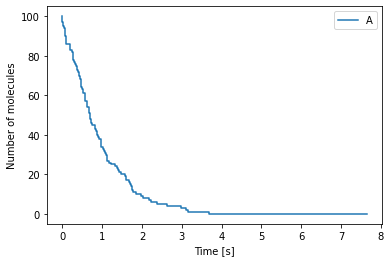
Chemical master equation example 1

We start with the following chemical reaction

\[A \xrightarrow{k} \emptyset \, ,\]

where molecules of species \(A\) decay at rate \(k \, [s^{-1}]\). The Python code for this simulation is as follows:

# Import pystospa
import pystospa as ss

# Create voxel object. Arguments: vector of number of molecules, size of the voxel
initial_num = [100]  # number of molecules of species A
domain_size = 10.0  # size of the domain in m^3
v = ss.Voxel(initial_num, domain_size)

# Create reaction object.
# Arguments: reaction rate, propensity func, stoichiometry vector
k = 1.0
propensity = lambda num_mols, area : num_mols[0]
stoch = [-1]
r = ss.Reaction(k, propensity, stoch)

# Add a reaction to a voxel
v.add_reaction(r)

# Pass the voxel with the reaction(s) to the simulator object
s = ss.Simulator([v])
# Run the simulation. Arguments: path to output file, time step, number of steps
s.run("cme_example.dat", 0.01, 500)

The output from the above simulation can be visualised using Python’s matplotlib module

import numpy as np
import matplotlib.pyplot as plt

# Read the file containing the data
data = np.loadtxt("cme_example.dat")
time = data[:, 0]  # Time points
num_A = data[:, 1]  # Number of molecules of A

# Plot of the data
fig, ax = plt.subplots()
ax.step(time, num_A, label="A")
ax.set_xlabel("Time [s]")
ax.set_ylabel("Number of molecules")
ax.legend()
plt.show()

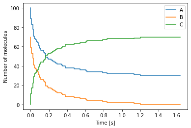
Chemical master equation example 2

As a second example of a chemical reaction system that StoSpa2 can simulate, we consider the following chemical reaction

\[A + B \xrightarrow{k} C \, ,\]

where a molecule of species \(A\) and a molecule of species \(B\) react to produce a molecule of species \(C\) at rate \(k \, [m^3 \, s^{-1}]\). The Python code for this reaction is as follows:

import pystospa as ss

# Create voxel object. Arguments: vector of number of molecules, size of the voxel
initial_num = [100, 70, 0]  # number of molecules of A, B and C repectively
domain_size = 10.0  # size of the domain in m^3
v = ss.Voxel(initial_num, domain_size)

# Create reaction object for reaction A + B -> C.
# Arguments: reaction rate, propensity func, stoichiometry vector
k = 1.0
propensity = lambda num_mols, length : num_mols[0]*num_mols[1]/length
stoch = [-1, -1, 1]
r = ss.Reaction(k, propensity, stoch)

# Add a reaction to a voxel
v.add_reaction(r)

# Pass the voxel with the reaction(s) to the simulator object
s = ss.Simulator([v])

# Run the simulation. Arguments: path to output file, time step, number of steps
s.run("cme_example_2.dat", 0.01, 500)

The output from the above simulation can be visualised using the Python code shown below:

import numpy as np
import matplotlib.pyplot as plt

# Read the file containing the data
data = np.loadtxt("cme_example_2.dat")
time = data[:, 0]
num_A = data[:, 1]
num_B = data[:, 2]
num_C = data[:, 3]

# Plot of the data
fig, ax = plt.subplots()
ax.step(time, num_A, label="A")
ax.step(time, num_B, label="B")
ax.step(time, num_C, label="C")
ax.set_xlabel("Time [s]")
ax.set_ylabel("Number of molecules")
ax.legend()
plt.show()

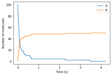
Chemical master equation example 3

Now, let us consider the following chemical reaction

\[A + A \xrightarrow{k} B \, ,\]

where two molecules of species \(A\) react at rate \(k \, [m^3\, s^{-1}]\) to produce a molecule of species \(B\).

import pystospa as ss

# Create voxel object. Arguments: vector of number of molecules, size of the voxel
initial_num = [100, 0]  # number of molecule of species A and B respectively
domain_size = 10.0  # size of the domain in m^3
v = ss.Voxel(initial_num, domain_size)

# Create reaction object for reaction A + A -> B.
# Arguments: reaction rate, propensity func, stoichiometry vector
k = 1.0
propensity = lambda num_mols, area : num_mols[0]*(num_mols[0] - 1)/area
stoch = [-2, 1]
r = ss.Reaction(k, propensity, stoch)

# Add a reaction to a voxel
v.add_reaction(r)

# Pass the voxel with the reaction(s) to the simulator object
s = ss.Simulator([v])

# Run the simulation. Arguments: path to output file, time step, number of steps
s.run("cme_example_3.dat", 0.01, 500)

After running the above code, we plot the data from the simulation as follows:

import numpy as np
import matplotlib.pyplot as plt

# Read the file containing the data
data = np.loadtxt("cme_example_3.dat")
time = data[:, 0]
num_A = data[:, 1]
num_B = data[:, 2]

# Plot of the data
fig, ax = plt.subplots()
ax.step(time, num_A, label="A")
ax.step(time, num_B, label="B")
ax.set_xlabel("Time [s]")
ax.set_ylabel("Number of molecules")
ax.legend()
plt.show()

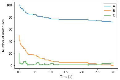
Chemical master equation example 4

The Last example of running simulations of a chemical reactions using the chemical master equation framework is the follwing:

\[A + B \xrightarrow{k_1} C \, , \quad B + 2C \xrightarrow{k_2} \emptyset \, ,\]

where we consider two reactions: one happening at rate \(k_1 \, [m^3\, s^{-1}]\) and the other happening at rate \(k_2 \, [m^6\, s^{-1}]\)

import pystospa as ss

# Create voxel object. Arguments: vector of number of molecules, size of the voxel
initial_num = [100, 50, 20]  # number of molecules of species A, B and C respectively
domain_size = 10.0  # size of the domain in m^3
v = ss.Voxel(initial_num, domain_size)

# Create reaction object for reaction A + B -> C.
# Arguments: reaction rate, propensity func, stoichiometry vector
k1 = 0.1
propensity1 = lambda num_mols, area : num_mols[0]*num_mols[1]/area
stoch1 = [-1, -1, 1]
r1 = ss.Reaction(k1, propensity1, stoch1)

# Create reaction object for reaction B + 2C -> 0. Arguments: reaction rate, propensity func, stoichiometry vector
k2 = 10.0
propensity2 = lambda num_mols, area : num_mols[1] * num_mols[2] * (num_mols[2] - 1) / (area**2)
stoch2 = [0, -1, -2]
r2 = ss.Reaction(k2, propensity2, stoch2)

# Add a reaction to the voxel
v.add_reaction(r1)
v.add_reaction(r2)

# Pass the voxel with the reaction(s) to the simulator object
s = ss.Simulator([v])

# Run the simulation. Arguments: path to output file, time step, number of steps
s.run("cme_example_4.dat", 0.01, 500)

The Python code below can be used to plot the output of the resulting simulation:

import numpy as np
import matplotlib.pyplot as plt

# Read the file containing the data
data = np.loadtxt("cme_example_4.dat")
time = data[:, 0]
num_A = data[:, 1]
num_B = data[:, 2]
num_C = data[:, 3]

# Plot of the data
fig, ax = plt.subplots()
ax.step(time, num_A, label="A")
ax.step(time, num_B, label="B")
ax.step(time, num_C, label="C")
ax.set_xlabel("Time [s]")
ax.set_ylabel("Number of molecules")
ax.legend()
plt.show()

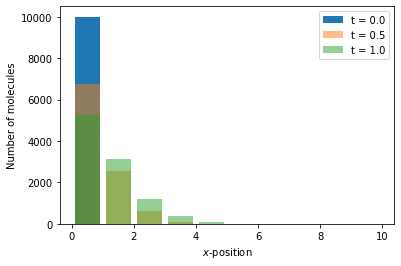
Reaction-diffusion master equation example 1

For a simple example of a simulation within reaction-diffusion master equation framework, we consider a one-dimensional domain \([0, 10]\), discretised into 10 voxels and we model the diffusion as a jump process between neighbouring voxels

\[A_1 \stackrel{d}{\rightleftharpoons} A_2 \stackrel{d}{\rightleftharpoons} A_3 \stackrel{d}{\rightleftharpoons} ... \stackrel{d}{\rightleftharpoons} A_{10} \, ,\]

where \(A_i\) is the the number of moleules in voxel \(i\). The Python code to simulate this system is as follows:

import pystospa as ss

# Create a vector of voxel objects. Voxel arguments: vector of number of molecules, size of the voxel
initial_num = [10000]  # initial number of molecules in the left-most voxel
voxel_size = 1.0  # size of a voxel in m^3
domain = [ss.Voxel(initial_num, voxel_size)]
# We add nine voxels with no molecules
for i in range(9):
    domain.append(ss.Voxel([0], voxel_size))

# Create and add the reaction objects
d = 1.0  # diffusion rate
propensity = lambda num_mols, length : num_mols[0]
stoch = [-1]
for i in range(9):
    # Add diffusion jump to the right from voxel i to voxel i+1
    domain[i].add_reaction(ss.Reaction(d, propensity, stoch, i+1))
    # Add diffusion jump to the left from voxel i+1 to voxel i
    domain[i+1].add_reaction(ss.Reaction(d, propensity, stoch, i))

# Pass the voxels with the reaction(s) to the simulator object
s = ss.Simulator(domain)

# Run the simulation. Arguments: path to output file, time step, number of steps
s.run("rdme_example.dat", 0.01, 200)

The Python code below can be used to plot the output:

import numpy as np
import matplotlib.pyplot as plt

# Read the file containing the data
data = np.loadtxt("rdme_example.dat")
time = data[:, 0]
num_A = data[:, 1:]
x = np.arange(0.5, 10.5)

# We generate a canvas for the figure
fig, ax = plt.subplots()
ax.bar(x, num_A[0], label="t = {:.2}".format(time[0]))
ax.bar(x, num_A[50], label="t = {:.2}".format(time[50]), alpha=0.5)
ax.bar(x, num_A[100], label="t = {:.2}".format(time[100]), alpha=0.5)
ax.set_xlabel(r"$x$-position")
ax.set_ylabel("Number of molecules")
ax.legend()
plt.show()

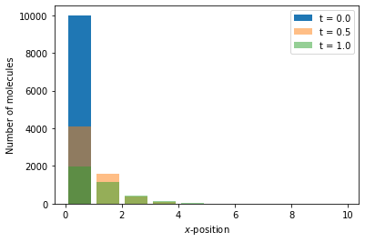
Reaction-diffusion master equation example 2

As a second example of a simulation within the reaction-diffusion master equation framework, we again consider a one-dimensional domain \([0, 10]\), discretised into 10 voxels. We model the diffusion as a jump process between neighbouring voxels

\[A_1 \stackrel{d}{\rightleftharpoons} A_2 \stackrel{d}{\rightleftharpoons} A_3 \stackrel{d}{\rightleftharpoons} ... \stackrel{d}{\rightleftharpoons} A_{10} \, ,\]

where \(A_i\) is the the number of moleules in voxel \(i\), and we include decay of molecules of A in each voxel, i.e.

\[A_i \xrightarrow{k} \emptyset \quad \text{for} \, i = 1, 2, 3, \ldots , 10 \, .\]

The Python code to simulate this system is as follows:

import pystospa as ss

# Create a vector of voxel objects. Voxel arguments: vector of number of molecules, size of the voxel
initial_num = [10000]
voxel_size = 1.0
domain = [ss.Voxel(initial_num, voxel_size)]
# We add nine voxels with no molecules
for i in range(9):
    domain.append(ss.Voxel([0], voxel_size))

# Create and add the reaction objects
d = 1.0  # diffusion rate
k = 1.0  # decay rate
propensity = lambda num_mols, length : num_mols[0]
stoch = [-1]
for i, vox in enumerate(domain):
    # Add diffusion jump to the right from voxel i to voxel i+1 (if one exists)
    if i < len(domain)-1: vox.add_reaction(ss.Reaction(d, propensity, stoch, i+1))
    # Add diffusion jump to the left from voxel i+1 to voxel i (if one exists)
    if i > 0: vox.add_reaction(ss.Reaction(d, propensity, stoch, i-1))
    vox.add_reaction(ss.Reaction(k, propensity, stoch))

# Pass the voxels with the reaction(s) to the simulator object
s = ss.Simulator(domain)

# Run the simulation. Arguments: path to output file, time step, number of steps
s.run("rdme_example_2.dat", 0.01, 200)

Something to note in the above code is that we define only one propensity function. This is due to the fact that the propensity functions for the diffusion reaction and the decay reaction have the same form (i.e. they are both first order reactions).

The output of a simulation can be visualised using the code below where we show the number of molecuels of species \(A\) at three times:

import numpy as np
import matplotlib.pyplot as plt

# Read the file containing the data
data = np.loadtxt("rdme_example_2.dat")
time = data[:, 0]
num_A = data[:, 1:]
x = np.arange(0.5, 10.5)

# We generate a canvas for the figure
fig, ax = plt.subplots()
ax.bar(x, num_A[0], label="t = {:.2}".format(time[0]))
ax.bar(x, num_A[50], label="t = {:.2}".format(time[50]), alpha=0.5)
ax.bar(x, num_A[100], label="t = {:.2}".format(time[100]), alpha=0.5)
ax.set_xlabel(r"$x$-position")
ax.set_ylabel("Number of molecules")
ax.legend()
plt.show()

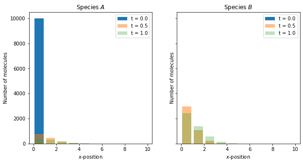
Reaction-diffusion master equation example 3

As a third example of a simulation within reaction-diffusion master equation framework, we again consider a one-dimensional domain \([0, 10]\), discretised into 10 voxels and we model the diffusion as a jump process

\[A_1 \stackrel{d}{\rightleftharpoons} A_2 \stackrel{d}{\rightleftharpoons} A_3 \stackrel{d}{\rightleftharpoons} ... \stackrel{d}{\rightleftharpoons} A_{10} \, ,\]

where \(A_i\) is the the number of moleules in voxel \(i\), but we include the following reaction:

\[A_i + A_i \xrightarrow{k} B_i \quad \text{for} \, i = 1, 2, 3, \ldots , 10 \, ,\]

where \(B_i\) is the number of molecules of species \(B\) in voxel \(i\). The Python code to simulate this system is as follows:

import pystospa as ss

# Create a vector of voxel objects. Voxel arguments: vector of number of molecules, size of the voxel
initial_num = [10000, 0]
voxel_size = 1.0
domain = [ss.Voxel(initial_num, voxel_size)]
# We add nine voxels with no molecules
for i in range(9):
    domain.append(ss.Voxel([0, 0], voxel_size))

# Create and add the reaction objects
d = 1.0  # diffusion rate
k = 0.001
prop_diff_A = lambda num_mols, length : num_mols[0]
prop_diff_B = lambda num_mols, length : num_mols[1]
prop_other = lambda num_mols, length : num_mols[0] * (num_mols[0] - 1) / length
stoch_diff_A = [-1, 0]
stoch_diff_B = [0, -1]
stoch_other = [-2, 1]
for i, vox in enumerate(domain):
    # Add diffusion jump to the right from voxel i to voxel i+1 (if one exists)
    if i < len(domain)-1:
        vox.add_reaction(ss.Reaction(d, prop_diff_A, stoch_diff_A, i+1))
        vox.add_reaction(ss.Reaction(d, prop_diff_B, stoch_diff_B, i+1))
    # Add diffusion jump to the left from voxel i+1 to voxel i (if one exists)
    if i > 0:
        vox.add_reaction(ss.Reaction(d, prop_diff_A, stoch_diff_A, i-1))
        vox.add_reaction(ss.Reaction(d, prop_diff_B, stoch_diff_B, i-1))
    vox.add_reaction(ss.Reaction(k, prop_other, stoch_other))

# Pass the voxels with the reaction(s) to the simulator object
s = ss.Simulator(domain)

# Run the simulation. Arguments: path to output file, time step, number of steps
s.run("rdme_example_3.dat", 0.01, 200)

Now with two species within the system, we plot the number of molecules of each species (\(A\) and \(B\)) in separate plots using the code below:

import numpy as np
import matplotlib.pyplot as plt

# Read the file containing the data
data = np.loadtxt("rdme_example_3.dat")
time = data[:, 0]
num_A = data[:, 1::2]
num_B = data[:, 2::2]
x = np.arange(0.5, 10.5)

# We generate a canvas for the figure
fig, axs = plt.subplots(1, 2, figsize=(10, 5), sharey=True)
titles = [r"Species $A$", r"Species $B$"]
for i, num in enumerate([num_A, num_B]):
    axs[i].bar(x, num[0], label="t = {:.2}".format(time[0]))
    axs[i].bar(x, num[50], label="t = {:.2}".format(time[50]), alpha=0.5)
    axs[i].bar(x, num[100], label="t = {:.2}".format(time[100]), alpha=0.3)
    axs[i].set_xlabel(r"$x$-position")
    axs[i].set_ylabel("Number of molecules")
    axs[i].set_title(titles[i])
    axs[i].legend()
plt.show()

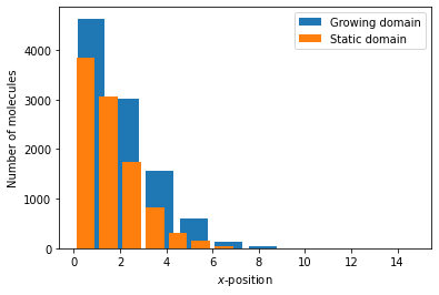
Reaction-diffusion master equation example 4

StoSpa2 also allows for stochastic simulations on uniformly growing domains. Consider the system

\[A_1 \stackrel{d}{\rightleftharpoons} A_2 \stackrel{d}{\rightleftharpoons} A_3 \stackrel{d}{\rightleftharpoons} ... \stackrel{d}{\rightleftharpoons} A_{10} \, ,\]

where \(A_i\) is the the number of molecules of species A in voxel \(i\), and molecules of A diffuse on the growing domain \(\Omega(t) = [0, L(t)]\), where \(L(t) = L_0 e^{rt}\). Then the Python code for this simulation, assuming that \(L_0 = 10\) and \(r = 0.2\), is as follows:

import pystospa as ss

# Create a vector of voxel objects. Voxel arguments: vector of number of molecules, size of the voxel
initial_num = [10000]
voxel_size = 1.0
growth = lambda t : np.exp(0.2 * t)
domain = [ss.Voxel(initial_num, voxel_size, growth)]
# We add nine voxels with no molecules
for i in range(9):
    domain.append(ss.Voxel([0], voxel_size, growth))

# Create and add the reaction objects
d = 1.0  # diffusion rate
propensity = lambda num_mols, length : num_mols[0]
stoch = [-1]
for i in range(9):
    # Add diffusion jump to the right from voxel i to voxel i+1
    domain[i].add_reaction(ss.Reaction(d, propensity, stoch, i+1))
    # Add diffusion jump to the left from voxel i+1 to voxel i
    domain[i+1].add_reaction(ss.Reaction(d, propensity, stoch, i))

# Pass the voxels with the reaction(s) to the simulator object
s = ss.Simulator(domain)

# Run the simulation. Arguments: path to output file, time step, number of steps
s.run("rdme_example_4.dat", 0.01, 200)

The main difference between the above code and the code in the reaction-diffusion master equation example 1 is that we add a lambda function for the growth of the domain to the constructor of the voxels

ss.Voxel(initial_num, voxel_size, growth)

where growth = lambda t : np.exp(0.2 * t). The output can be visualised using the following Python code:

import numpy as np
import matplotlib.pyplot as plt

# Read the file containing the data
data = np.loadtxt("rdme_example_4.dat")
data_static = np.loadtxt("rdme_example.dat")
time = data[:, 0]
num_A = data[:, 1:]
num_A_static = data_static[:, 1:]
x = np.arange(0.5, 10.5)
growth = lambda t : np.exp(0.2 * t)

# We generate a canvas for the figure
fig, ax = plt.subplots()
ax.bar(x*growth(time[199]), num_A[199], label="Growing domain", width=0.8*growth(time[199]))
ax.bar(x, num_A_static[199], label="Static domain")
ax.set_xlabel(r"$x$-position")
ax.set_ylabel("Number of molecules")
ax.legend()
plt.show()

C++ examples

Chemical master equation

As first example, let us consider the following chemical reaction

\[A \xrightarrow{k} \emptyset \, ,\]

happening at some rate \(k \, [s^{-1}]\). We can simulate this chemical system with the following code:

#include "simulator.hpp"

int main() {
    // Create voxel object. Arguments: vector of number of molecules, size of the voxel
    std::vector<unsigned> initial_num = {100};  // number of molecules of species A
    double domain_size = 10.0;  // size of the domain in cm
    StoSpa2::Voxel v(initial_num, domain_size);

    // Create reaction object.
    // Arguments: reaction rate, propensity func, stoichiometry vector
    double k = 1.0;
    auto propensity = [](const std::vector<unsigned>& num_mols, const double& area) { return num_mols[0]; };
    std::vector<int> stoch = {-1};
    StoSpa2::Reaction r(k, propensity, {-1});

    // Add a reaction to a voxel
    v.add_reaction(r);

    // Pass the voxel with the reaction(s) to the simulator object
    StoSpa2::Simulator s({v});

    // Run the simulation. Arguments: path to output file, time step, number of steps
    s.run("cme_example.dat", 0.01, 500);
}

In the first segment of the code we define the domain of the system using a single Voxel object, by specifiying the input arguments of the Voxel object, then initialising the Voxel object as follows:

std::vector<unsigned> initial_num = {100};  // number of molecules of species A
double domain_size = 10.0;  // size of the domain in cm
StoSpa2::Voxel v(initial_num, domain_size);

Next, we create the reaction object by specifying the reaction rate (\(k\)), the propensity function and the stoichiometry vector for the decay reaction, which we then use to create a Reaction object in the segment below:

double k = 1.0;
auto propensity = [](const std::vector<unsigned>& num_mols, const double& area) { return num_mols[0]; };
std::vector<int> stoch = {-1};
StoSpa2::Reaction r(k, propensity, {-1});

After creating the Reaction object, we can pass it to the previously created Voxel object:

v.add_reaction(r);

Finally, we create the Simulator object, whose run function is used to run the simulation:

StoSpa2::Simulator s({v});
s.run("cme_example.dat", 0.01, 500);

We can plot the output of the simulation using the following Python code:

import numpy as np
import matplotlib.pyplot as plt

# Open the file containing the data
data = np.loadtxt("cme_example.dat")
time = data[:, 0]  # Time points
num_A = data[:, 1]  # Number of molecules of A

# Plot the data and label the axes
fig, ax = plt.subplots()
ax.step(time, num_A, label="A")
ax.set_xlabel("Time [s]")
ax.set_ylabel("Number of molecules")
ax.legend()
plt.show()

Reaction-diffusion master equation example

To show how the StoSpa2 can be used to run simulations within the reaction-diffusion master equation framework we use the example of a one-dimensional domain \([0, 10]\), discretised into \(10\) voxels and we model the diffusion as a jump process of the form

\[A_1 \stackrel{d}{\rightleftharpoons} A_2 \stackrel{d}{\rightleftharpoons} A_3 \stackrel{d}{\rightleftharpoons} ... \stackrel{d}{\rightleftharpoons} A_{10} \, ,\]

where \(A_i\) is the the number of moleules in voxel \(i\). The C++ code for such a system is as follows:

#include "simulator.hpp"

using namespace StoSpa2;

int main() {

    // Create a vector of voxel objects. Voxel arguments: vector of number of molecules, size of the voxel
    std::vector<unsigned> initial_num = {10000};  // number of molecules of A in left-most voxel
    double voxel_size = 1.0;  // length of a voxel in cm
    // First create nine empty voxels
    std::vector<Voxel> vs = std::vector<Voxel>(9, Voxel({0}, voxel_size));
    // Then add the non-empty voxel at the beginning
    vs.insert(vs.begin(), Voxel(initial_num, voxel_size));

    double d = 1.0;  // diffusion rate
    auto propensity = [](const std::vector<unsigned>& num_mols, const double& area) { return num_mols[0]; };
    std::vector<int> stoch = {-1};
    // Create and add the reaction objects
    for (unsigned i=0; i<vs.size()-1; i++) {
        // Add diffusion jump to the right from voxel i to voxel i+1
        vs[i].add_reaction(Reaction(d, propensity, stoch, i+1))
        // Add diffusion jump to the left from voxel i+1 to voxel i
        vs[i+1].add_reaction(Reaction(d, propensity, stoch, i));
    }

    // Pass the voxels with the reaction(s) to the simulator object
    Simulator s(vs);

    // Run the simulation. Arguments: path to output file, time step, number of steps
    s.run("rdme_example.dat", 0.01, 500);
}

In the first segment of the code above, we create ten Voxel objects that partition the domain into equally-sized segments and we populate the left-most voxel with \(10000\) molecules of species \(A\), i.e. \(A_1 = 10000\):

// Create a vector of voxel objects. Voxel arguments: vector of number of molecules, size of the voxel
std::vector<unsigned> initial_num = {10000};  // number of molecules of A in left-most voxel
double voxel_size = 1.0;  // length of a voxel in cm
// First create nine empty voxels
std::vector<Voxel> vs = std::vector<Voxel>(9, Voxel({0}, voxel_size));
// Then add the non-empty voxel at the beginning
vs.insert(vs.begin(), Voxel(initial_num, voxel_size));

In the following segment, we create Reaction objects that simulate the diffusion of molecules of \(A\) as jumps between adjacent voxels and pass them immediately to the appropriate voxels:

double d = 1.0;  // diffusion rate
auto propensity = [](const std::vector<unsigned>& num_mols, const double& area) { return num_mols[0]; };
std::vector<int> stoch = {-1};
// Create and add the reaction objects
for (unsigned i=0; i<vs.size()-1; i++) {
    // Add diffusion jump to the right from voxel i to voxel i+1
    vs[i].add_reaction(Reaction(d, propensity, stoch, i+1))
    // Add diffusion jump to the left from voxel i+1 to voxel i
    vs[i+1].add_reaction(Reaction(d, propensity, stoch, i));
}

And finally, we create a Simlator object by initialising it with the vector of Voxel objects, followed by using the run function to run the simulation:

// Pass the voxels with the reaction(s) to the simulator object
Simulator s(vs);

// Run the simulation. Arguments: path to output file, time step, number of steps
s.run("rdme_example.dat", 0.01, 500);

We can plot the output of the simulation using the following Python code:

import numpy as np
import matplotlib.pyplot as plt

# Read the file containing the data
data = np.loadtxt("rdme_example.dat")
time = data[:, 0]
num_A = data[:, 1:]
x = np.arange(0.5, 10.5)

# We generate a canvas for the figure
fig, ax = plt.subplots()
ax.bar(x, num_A[0], label="t = {:.2}".format(time[0]))
ax.bar(x, num_A[50], label="t = {:.2}".format(time[50]), alpha=0.5)
ax.bar(x, num_A[100], label="t = {:.2}".format(time[100]), alpha=0.5)
ax.set_xlabel(r"$x$-position")
ax.set_ylabel("Number of molecules")
ax.legend()
plt.show()